[ML-05]Logistic Regression
5. Logistic Regression
5.1 Logistic Regression
what?
- 회귀 방정식을 통해 데이터를 분류하는 모델
- categorical 변수의 경우 연속형 변수와 달리 중간값을 가지지 않으므로 일반적인 linear regression과 다른 접근법이 필요하다.
- regression 모델을 0~1 사이의 값을 가지도록 변형하면 logistic function과 같은 형태가 된다.

- \(h_\theta(x) = \frac 1 {1+e^{-\theta^Tx}}\), \((\theta^Tx) = \theta + \theta_1x_1 + ... + \theta_nx_n\)으로 regression 모델이다.

- 여기서 regression 모델은 데이터를 구분짓는 decision boundary를 형성한다.
- logistic regression은 항상 0과 1 사이의 확률값을 반환한다.
- \(\theta^Tx \ge 0\) means \(h_\theta(x) \ge 0.5\) ==> y = 1
- \(\theta^Tx \le 0\) means \(h_\theta(x) \le 0.5\) ==> y = 0
 </img>
 - regression 모델과 다른 loss function을 사용한다.
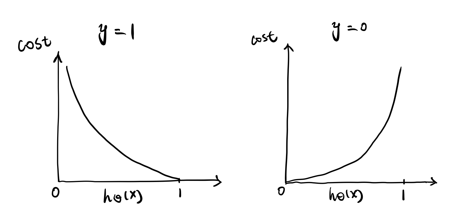
- \[J(\theta)_{logistic} = \frac 1 m {\sum_{i=1}^M((y_ilog(h_\theta(x_i))) + (1-y_i)log(1-h_\theta(x_i)))}\]
- logistic regression의 loss function은 예측값과 실제 데이터가 다를 때 penalty를 높히는 형식으로 구성되어 있다. 예를 들어 실제 데이터는 1인데 0으로 예측한 경우 높은 penalty가 부가되어 학습이 잘 되도록 유도한다.
 </img>
why?
- 연산량이 많지 않아 시간적인 효율성을 가진다.
- 가볍고 모델을 학습시키기 용이하다.
why not?
- linear regression과 마찬가지로 선형 관계에 있는 경우에만 사용 가능하다.
- 연속형 데이터에 대한 예측이 불가능하다.
- overfitting될 가능성이 높다.
how?
Input
1)Data\({(x_i, y_i)}\), M rows(data) and 1 column(feature)
2) Model : \(J(\theta)_{logistic} = \frac 1 m {\sum_{i=1}^M((y_ilog(h_\theta(x_i))) + (1-y_i)log(1-h_\theta(x_i)))}\)
3) Loss function \(J(\theta) = {\frac 1 M}\sum_{i=1}^M (y_i - \hat{y_i})^2\)
step 1. initialize parameters \(\theta\) for Model
step 2. find optimal paramters
1) gradient descent를 통해 파라미터 \(\theta\)에 대해서 최적의 값을 찾는다.
2) \(\theta\) 값을 logistic regression 모델에 적용하여 확률값을 찾는다.
3) 확률값에 따른 범주 \(\hat{y_i}\) 를 얻는다. 이진분류의 경우 \(h_\theta(x) \ge 1/2\) 이면 \(\hat{y_i} = 1\), \(h_\theta(x) < 1/2\) 이면
step 3. ouput : 데이터에 대한 예측 범주 \(\hat{y_i}\)
Code usage
from sklearn.linear_model import LogisticRegression
from sklearn.datasets import load_iris
import numpy as np

# load dataset
iris = load_iris()

# petal length, petal width만 사용
X = iris["data"][:, (2, 3)]  # petal length, petal width
y = (iris["target"] == 2).astype(np.int)

# model selection
# sklearn은 default값으로 Logistic Regression에 규제항을 추가한다.
# solver는 optimization 방법에 해당한다.
# C는 규제의 정도를 정하는 파라미터로 값이 작을수록 더 큰 규제가 적용된다
log_reg = LogisticRegression(solver='liblinear', C=10**10, random_state=42)
log_reg.fit(X, y)

x0, x1 = np.meshgrid(
        np.linspace(2.9, 7, 500).reshape(-1, 1),
        np.linspace(0.8, 2.7, 200).reshape(-1, 1),
    )
X_new = np.c_[x0.ravel(), x1.ravel()]

y_proba = log_reg.predict_proba(X_new) # 각 범주에 속할 확륡값
y_pred = log_reg.predict(X_new)  # 예측 범주
5.2 Softmax Regression
what?
- 다중 분류를 위해 사용되는 알고리즘으로 logistic regression을 결합한 결과와 같다.
- regression을 통해 얻어진 각 data에 대한 수치를 softmax function을 통해 확률값으로 sclaing해준다.
- softmax function $S(y_i) = {exp(y_i)}/{\sum_{i=1}^{M}(exp(y_i))}$$
- loss function으로는 cross-entropy를 사용한다. 예측한 범주와 실제 범주값의 차이를 토대로 잘못 예측한 경우 penalty를 주는 방식으로 logistic regression의 loss function과 유사하다.
- Loss function \(J(\theta)_{softmax} = \frac 1 m {\sum_{i=1}^M(y_i) * -log(S(y_i))}\)

why?
- logistic regression과 동일
why not?
- logistic regression과 동일
how?
Input
1)Data{(\(x_i, y_i\))}, M rows(data) and 1 column(feature), K categories 2) Model : \(J(\theta)_{logistic} = \frac 1 m {\sum_{i=1}^M((y_ilog(h_\theta(x_i))) + (1-y_i)log(1-h_\theta(x_i)))}\)
3) Loss function \(J(\theta)_{softmax} = \frac 1 m {\sum_{i=1}^M(y_i) * -log(S(y_i))}\)
step 1. initialize parameters \(\theta\) for Model
step 2.
1) for k = 1 to K regression을 적용하여 각 데이터에 대한 수치를 얻는다.
2) softmax function을 적용하여 각 데이터에 대한 범주 벡터를 얻는다.
3) cross-entropy loss function을 토대로 gradient descent를 진행하여 데이터에 대한 예측 범주 \(\hat{y_i}\)를 얻는다.
step 3. ouput : 데이터에 대한 예측 범주 \(\hat{y_i}\)
code usage
from sklearn.linear_model import LogisticRegression
from sklearn.datasets import load_iris
import numpy as np

# load dataset
iris = load_iris()

# petal length, petal width만 사용
X = iris["data"][:, (2, 3)]
y = iris["target"]

# model selection
# multi_class 지정해주기
softmax_reg = LogisticRegression(multi_class="multinomial",solver="lbfgs", C=10, random_state=42)
softmax_reg.fit(X, y)

x0, x1 = np.meshgrid(
        np.linspace(0, 8, 500).reshape(-1, 1),
        np.linspace(0, 3.5, 200).reshape(-1, 1),
    )
X_new = np.c_[x0.ravel(), x1.ravel()]

# predict categories
y_proba = softmax_reg.predict_proba(X_new)
y_pred = softmax_reg.predict(X_new)

print(y_proba)
print(y_pred)
Reference
핸즈온 머신러닝
Coursera : Machine Learning by Andrew Ng
logistic regresion의 장단점
logistic regression 최적화 방법
logistic regression solver 파라미터에 대한 설명
softmax regression 설명